Maximum temperature for year using Spark SQL

In the previous blog, we looked at how find out the maximum temperature of each year from the weather dataset. Below is the code for the same using Spark SQL which is a layer on top of Spark. SQL on Spark was supported using Shark which is being replaced by Spark SQL. Here is a nice blog from DataBricks on the future of SQL on Spark.

import re
import sys

from pyspark import SparkContext
from pyspark.sql import SQLContext, Row

#function to extract the data from the line
#based on position and filter out the invalid records
def extractData(line):
    val = line.strip()
    (year, temp, q) = (val[15:19], val[87:92], val[92:93])
    if (temp != "+9999" and re.match("[01459]", q)):
        return [(year, temp)]
    else:
        return []

logFile = "hdfs://localhost:9000/user/bigdatavm/input"

#Create Spark Context and SQL Context with the master details and the application name
sc = SparkContext("spark://bigdata-vm:7077", "max_temperature")
sqlContext = SQLContext(sc)

#Create an RDD from the input data in HDFS
weatherData = sc.textFile(logFile)

#Transform the data to extract/filter and then map it to a row
temperature_data = weatherData.flatMap(extractData).map(lambda p: Row(year=p[0], temperature=int(p[1])))

#Infer the schema, and register the SchemaRDD as a table.
temperature_data = sqlContext.inferSchema(temperature_data)
temperature_data.registerTempTable("temperature_data")

#SQL can be run over SchemaRDDs that have been registered as a table.
#Filtering can be done in the SQL using a where clause or in a py function as done in the extractData()
max_temperature_per_year = sqlContext.sql("SELECT year, MAX(temperature) FROM temperature_data GROUP BY year")

#Save the RDD back into HDFS
max_temperature_per_year.saveAsTextFile("hdfs://localhost:9000/user/bigdatavm/output")

Maximum temperature for year using Spark/Python

Hadoop – The Definitive Guide revolves around the example of finding the maximum temperature for a particular year from the weather data set. The code for the same is here and the data here. Below is the Spark code implemented in Python for the same.

import re
import sys

from pyspark import SparkContext

#function to extract the data from the line
#based on position and filter out the invalid records
def extractData(line):
    val = line.strip()
    (year, temp, q) = (val[15:19], val[87:92], val[92:93])
    if (temp != "+9999" and re.match("[01459]", q)):
        return [(year, temp)]
    else:
        return []

logFile = "hdfs://localhost:9000/user/bigdatavm/input"

#Create Spark Context with the master details and the application name
sc = SparkContext("spark://bigdata-vm:7077", "max_temperature")

#Create an RDD from the input data in HDFS
weatherData = sc.textFile(logFile)

#Transform the data to extract/filter and then find the max temperature
max_temperature_per_year = weatherData.flatMap(extractData).reduceByKey(lambda a,b : a if int(a) > int(b) else b)

#Save the RDD back into HDFS
max_temperature_per_year.saveAsTextFile("hdfs://localhost:9000/user/bigdatavm/output")

The map function during the transformation is similar to the map function in the MR model and reduceByKey transformation is similar to the reduce function in the MR model.

In the future blogs, we will see how to perform complex processing using the other transformations and actions provided by Spark.

Hadoop/MR vs Spark/RDD WordCount program

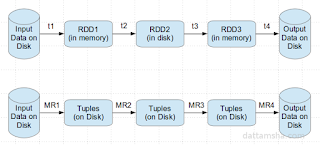
Apache Spark provides an efficient way for solving iterative algorithms by keeping the intermediate data in the memory. This avoids the overhead of R/W of the intermediate data from the disk as in the case of MR.

Also, when running the same operation again and again, data can be cached/fetched from the memory without performing the same operation again. MR is stateless, lets say a program/application in MR has been executed 10 times, then the whole data set has to be scanned 10 times.

Also, namesake MR supports only Map and Reduce operations and everything (join, groupby etc) has to be fit into the Map and Reduce model, which might not be the efficient way. Spark supports a couple of other transformations and actions besides just Map and Reduce as mentioned here and here.

Spark code is also compact when compared to the MR code. Below is the program for performing the WordCount using Python in Spark.

from pyspark import SparkContext

logFile = "hdfs://localhost:9000/user/bigdatavm/input"

sc = SparkContext("spark://bigdata-vm:7077", "WordCount")

textFile = sc.textFile(logFile)

wordCounts = textFile.flatMap(lambda line: line.split()).map(lambda word: (word, 1)).reduceByKey(lambda a, b: a+b)

wordCounts.saveAsTextFile("hdfs://localhost:9000/user/bigdatavm/output")

and the same in MR model using Hadoop is a bit verbose as shown below.

package org.apache.hadoop.examples;

import java.io.IOException;
import java.util.StringTokenizer;

import org.apache.hadoop.conf.Configuration;
import org.apache.hadoop.fs.Path;
import org.apache.hadoop.io.IntWritable;
import org.apache.hadoop.io.Text;
import org.apache.hadoop.mapreduce.Job;
import org.apache.hadoop.mapreduce.Mapper;
import org.apache.hadoop.mapreduce.Reducer;
import org.apache.hadoop.mapreduce.lib.input.FileInputFormat;
import org.apache.hadoop.mapreduce.lib.input.FileSplit;
import org.apache.hadoop.mapreduce.lib.output.FileOutputFormat;
import org.apache.hadoop.util.GenericOptionsParser;

public class WordCount {

    public static class TokenizerMapper extends
        Mapper<Object, Text, Text, IntWritable> {

        private final static IntWritable one = new IntWritable(1);
        private Text word = new Text();

        public void map(Object key, Text value, Context context)
            throws IOException, InterruptedException {
            StringTokenizer itr = new StringTokenizer(value.toString());
            while (itr.hasMoreTokens()) {
                word.set(itr.nextToken());
                context.write(word, one);
            }
        }
    }

    public static class IntSumReducer extends
        Reducer<Text, IntWritable, Text, IntWritable> {

        private IntWritable result = new IntWritable();

        public void reduce(Text key, Iterable<Intwritable> values,
        Context context) throws IOException, InterruptedException {
            int sum = 0;
            for (IntWritable val : values) {
                sum += val.get();
            }
            result.set(sum);
            context.write(key, result);
        }
    }

    public static void main(String[] args) throws Exception {
        Configuration conf = new Configuration();
        String[] otherArgs = new GenericOptionsParser(conf, args)
            .getRemainingArgs();

        Job job = new Job(conf, "word count");

        job.setJarByClass(WordCount.class);

        job.setMapperClass(TokenizerMapper.class);
        job.setCombinerClass(IntSumReducer.class);
        job.setReducerClass(IntSumReducer.class);

        job.setOutputKeyClass(Text.class);
        job.setOutputValueClass(IntWritable.class);

        FileInputFormat.addInputPath(job, new Path(otherArgs[0]));
        FileOutputFormat.setOutputPath(job, new Path(otherArgs[1]));

        System.exit(job.waitForCompletion(true) ? 0 : 1);
    }
}

Here we looked into WordCount which is similar to HelloWorld program in terms of simplicity, for one to get started with a new concept/technology/language. In the future blogs, we will look into a little more advanced features in Spark.

Intersection of Big Data and IOT

Lately I had been blogging about IOT and Big Data. They go hand-in-hand. With the IOT devices feeding the data to the Big Data platforms on the Cloud to store/analyze the data and feed it back to the IOT devices. One such example is the Nest device bought by Google. Nest thermostat gathers the room temperature, sends it over to the Cloud over Wi-Fi, analytics done in the Cloud and fed back to the Nest again.

This is not something new, but had been there for quite some time. But, the conditions are moving towards more adoption of Big Data and IOT like cheap sensors, Cloud, cheaper and faster internet connections. Here is an article  from ZDNet on ten practical examples on the intersection of Big Data and IOT. For those who are interested in learning more, here (1, 2) are few more references from ZDNet.

I am yet to try it out, but here is a detailed article from IBM Developer Works on building a temperature sensor using Arduino Uno, putting the data in the Cloud and finally visualizing the data in a real time. Here is another article on how to integrate IOT with Azure.

Getting started with Apache Spark

With so much noise around Apache Spark, let's look into how to get started with Spark in local mode and execute a simple Scala program. A lot of complex combinations are possible, but we will look at the minimum steps required to get started with Spark.

Most of the Big Data softwares are developed with Linux as the platform and porting to Windows has been an after thought. It is interesting to see how Big Data on Windows will morph in the future. Spark can run on both Windows/Linux, but we will take Linux (Ubuntu 14.04 64-bit Desktop) into consideration. So, here are the steps:

1) Download and install Oracle VirtualBox as mentioned here.

2) Download and install Ubuntu as mentioned here as a guest OS.

3) Update the patches on Ubuntu from a terminal and reboot it.

sudo apt update;sudo apt-get dist-upgrade

4) Oracle Java doesn't come with Linux distributions, so has to be installed manually on top of Ubuntu as mentioned here.

5) Spark has been developed in Scala, so we need install Scala.

sudo apt-get install scala

6) Download Spark from here and extract it. Spark built with hadoop 1x or 2x will work, because HDFS is not being used in this context.

7) From the Spark installation folder start the Spark shell.

bin/spark-shell

8) Execute the below commands in the shell to load the README.md and count the number of lines in it.

val textFile = sc.textFile("README.md")

textFile.count()

What we have done is install Ubuntu as a guest OS and then install Spark on it. And finally run a simple Scala program in Spark local mode. There are much more advanced setups like running Spark program against data in HDFS, running Spark in stand alone, Mesos and YARN mode. We will look at them in the future blogs.

ASF (Apache Software Foundation) as a standards body

What is ASF all about?

For many Apache is synonymous to the Apache HTTP server, which is the backbone for serving the web pages. But, there is much more to Apache. It's a non profit organization (ASF - Apache Software Foundation) which provides an environment and a platform in which different companies and individuals work in an open and collaborative fashion towards a common goal of developing a good piece of software. Open means that all the work (architecture, design, coding, testing, documentation etc) happens in an open way and there are no secrets. Anyone can also download the code, make some changes, compile it and push it back.

It's possible for different companies and individuals like you and me to improve the code and contribute it back to the ASF. To maintain the quality of the software there is a process in place where the project committer will check the quality of the code contributed by someone and then add them to the code repository. The advantage of working in this model is that any improvements made by an individual or a company can be immediately absorbed by someone else. This is what working in a collaborative fashion means.

There are a lot of Big Data projects under the ASF like Hadoop, Hive, Pig, HBase, Cassandra and a lot of non Big Data projects like Tomcat, Log4J, Velocity, Struts. The projects usually start with Incubator status and then some of them move to the TLP status (Top Level Project). The code for the different projects can be accessed in a read only way from here.


How is Apache promoting standards?

OK, now we know how the Apache process works. The different companies and individuals work towards the common goal of creating good software. Now, lets look into why standards are important in software and how Apache is promoting the standards.

Those who travel internationally and carry at least one electronic item, face the problem with the different socket layout and the voltages in different countries. The plugs just don't fit in into the sockets and so is the need to carry multiple adapters. If there had been an international standard for the socket layout and the voltage, we wouldn't face this problem.

The same can be applied to software standards also. Software standards allow interoperability across different software stacks. As an example, a program written against one software can be easily ported to some other software if the standards are followed. One example is the JEE standards. An EJB written for JBoss can be easily ported to WebSphere with minimal or no changes.

In the case of Big Data stacks, the different Big Data companies take the software from the Apache Software foundation and improve on it. Some of the improvements can be better documentation,  better performance, bug fixes, better usability in terms of installation/monitoring/alerting.

The Apache code is the common base for the different Big Data distributions. Due to this reason the Apache code base and the different distributions like HDP, CDH etc provide more or less the same API to program against. This way Apache is acting as a standards body. For example a MapReduce program written against HDP distribution can be run against the other distributions with minimal or no changes.

Although Apache is not a standards body, it is still acting as one. Usually, a standards body is formed and they do develop standards and a reference implementation for the same. This is a painstaking process and some of the standards may not see the light of the day also. The advantage of working in the Apache fashion is that the standards are developed indirectly in a very quick fashion.

What is Dockers all about?

There had been a lot of noise about Docker. And there had been a raft of announcements (1, 2, 3) about the support for Docker in their products from different  companies. In this blog, we will look what Docker is all about, but before that we will look into what virtualization, LXC. In fact, Docker-Big Data integration also can be done.

What is Virtualization?

Virtualization allows to run multiple operating systems on a single machine. For this to happen virtualization software like Xen, KVM, HyperV, VMWare vSphere, VirtualBox has to be installed. Oracle VirtualBox is free and easy to setup. Once VirtualBox has been installed, multiple guest OS can be run on top of VirtualBox as shown below.

On top of the guest OS, applications can be installed. The main advantage of the above configuration is that the applications are isolated from each other. And also, resources can be allocated to the guest OS and a single application can’t dominate and use the underlying hardware resources completely and let the other applications starve for resources. The main disadvantage is each of the guest OS gets it’s own kernel and the file system and hence consume a lot of resources.

What is LXC?

LXC (Linux Containers) provide OS level virtualization and don’t need a complete OS to be installed as mentioned in the case of virtualization.

The main advantage of LXC is that they are light weight and there is little over head of running the applications on top of LXC instead of directly on top of the host OS. And also, LXC provides isolation between the different applications deployed in them and resources can also be allocated them.

LXC can be thought of light weight machines which consume less resources, are easy to start and on which applications can be deployed.

How does Docker fit into the entire thing?

LXCs are all interesting, but it’s not that easy to migrate an application on top of LXC from one environment to another (let’s say from development to QA to production) as there are a lot of dependencies between the application and the the underlying system.

Docker provides a platform, so that applications can be be built and packaged in a standardized way. The application built, will also include all the dependencies and so there is less friction moving from one environment to another environment. Also, Docker will try to abstract the resources required for the application, so that that application can run in different environments without any changes.

For those from a Java/JEE background, Docker applications can be considered similar to an EAR file which can be migrated from one environment to another without any changes as long as the proper standards are followed while creating the EAR file. The Java applications can make JNDI calls to discover services by name and so are not tied to a particular resource.

BTW, here is a nice documentation on Docker.

Consolidating the blogs

I have a few other web sites onlyubuntu.com (around Ubuntu) and dattamsha.com (around Big Data, IOT and related technologies) besides the current one. Over time it has become difficult to maintain multiple sites and also I had not been updating the other sites on a regular basis.

So, I decided to consolidate the sites to thecloudavenue.com (the current site). In this process, I would be moving the blogs from the other sites to this this site in a phase vise manner.

Happy reading !!!!

Snap Circuits Jr. from Elenco for kids

Lately I had been my hands-on with the RaspberryPi and Arduino prototype kits to get started with IOT (Internet Of Things). Being a graduate in Electrical and Electronics Engineering helped me in getting started quickly.

I built a car with 4 DC motors, control it using a TV remote control which emits IR (Infra Red) signal. The IR signal was captured by the IR sensor on the car. Based on the button pressed on the remote control an Arduino program controlled the speed of the motors. This made the car move in different directions. It was not too complicated, but was fun to build.

All the time I was building the car, my son used to tag with me asking questions on what the different parts were and how they function. To continue his interest in the same, I bought him a Snap Circuits Jr. SC-100 and he was more than happy to do different circuits with it. The Snap Circuits comes with different models like Snap Circuits SC-300, Snap Circuits PRO SC-500 and finally the Snap Circuits Extreme SC-750. The Snap Circuits can be upgraded easily. There is a Snap Circuits UC-30 Upgrade Kit SC-100 to SC-300 and others.

The Snap Circuits are a big rugged and don't get damaged very easily, the only thing which needs to be taken care is the polarity of the components when connecting. There is no need to solder, the different components snap with each other using the push buttons. Batteries are the only items which need to be bought separately. It comes with a manual/guide explaining the different components, trouble shooting tips, circuit diagrams etc which is really nice.

As the name says, connecting them is a snap and fun. Would very much recommend for those who want to get their kids started with electronics.

Comparing ORC vs Parquet Data Storage Formats using Hive

CSV is the most familiar way of storing the data. In this blog I will try to compare the performance aspects of the ORC and the Parquet formats. There is a lot of literature on what these are, so less focus on the same.

Similar to Parquet for storing the data in the column oriented format there is another format called ORC. Parquet had been aggressively promoted by Cloudera and ORC by Hortonworks. Here are some articles (1, 2) on Parquet vs ORC.

The CSV data can be converted into ORC and Parquet formats using Hive. These are the steps involved. The same steps are applicable to ORC also. Simply, replace Parquet with ORC. Behind the scenes a MapReduce job will be run which will convert the CSV to the appropriate format.

- Create a Hive table (ontime)
- Map the ontime table to the CSV data
- Create a Hive table ontime_parquet and specify the format as Parquet
- Move the table from the ontime table to the ontime_parquet table

In the previous blog, we have seen how to convert CSV into Parquet using Hive. The procedure is more or less for ORC, just replace the `STORED AS PARQUET` to `STORED AS ORC` in the table definition as shown below and also specify the compressions codec to use.

create external table ontime_orc_snappy (
  Year INT,
  Month INT,
  DayofMonth INT,
  DayOfWeek INT,
  DepTime  INT,
  CRSDepTime INT,
  ArrTime INT,
  CRSArrTime INT,
  UniqueCarrier STRING,
  FlightNum INT,
  TailNum STRING,
  ActualElapsedTime INT,
  CRSElapsedTime INT,
  AirTime INT,
  ArrDelay INT,
  DepDelay INT,
  Origin STRING,
  Dest STRING,
  Distance INT,
  TaxiIn INT,
  TaxiOut INT,
  Cancelled INT,
  CancellationCode STRING,
  Diverted STRING,
  CarrierDelay INT,
  WeatherDelay INT,
  NASDelay INT,
  SecurityDelay INT,
  LateAircraftDelay INT
) STORED AS PARQUET LOCATION '/user/bigdata/airline/input-orc-snappy-from-hive' TBLPROPERTIES ("orc.compress"="SNAPPY");

Then the data has to be moved from the regular Hive table (ontime) to the ontime_orc_snappy using the below command.

INSERT OVERWRITE TABLE ontime_parquet_gzip SELECT * FROM ontime;

The property name for the and the default properties are mentioned in the below table. When not using the default compression codec then the property can be set on the table using the TBLPROPERTIES as shown in the above table creation command. Note that ZLIB in ORC and GZIP in Parquet uses the same compression codec, just the property name is different.

 

Four tables need to be created in Hive for the combination of orc/parquet and snappy/zlib/gzip compression as shown below.

Now that the tables have been created, the data can be moved from the ontime table to the remaining four tables. Four folders in HDFS will be created as shown below.

One the four tables I ran two queries on all the four tables. The first query was of type aggregation to find the number of delayed flights per origin as shown below.

select Origin, count(*) from ontime_parquet_gzip where DepTime > CRSDepTime group by Origin;

The second query is to fetch all the columns in a single row as shown below.

select * from ontime_parquet_gzip where origin = 'LNY' and AirTime = 16;

Below is the comparison matrix which is of main interest.

Here are a few things which I want to highlight

- There is not much of storage savings when using using ORC and Parquet when using the same compression code like `SNAPPY vs SNAPPY` and `ZLIB vs GZIP`.

- The time for converting from CSV to ORC and Parquet format is very close, not much difference considering the total time it takes for the conversion.

- Hortonworks blog says that the ORC format provides much better compression ratio when compared to Parquet. This is a bit misleading as the default properties are being used, ZLIB for ORC and SNAPPY for Parquet. By making sure that both the formats use the compression codec, there is not much significant difference in the compression ratio as shown in the above matrix. So, it would be better to focus on the features.

- For aggregation queries like `time for the the delayed flights` there is not such a drastic difference. Both the ORC and Parquet formats perform considerably well when compared to the CSV format.

- While fetching all the columns for a single now using a condition like "where origin = 'LNY' and AirTime = 16;", ORC has an edge over Parquet because the ORC format has a light index along with each file. By using the indexes in ORC, the underlying MapRedeuce or Spark can avoid reading the entire block.

- The indexing in Parquet seems to be a good differentiator. Although the ORC has to create Index while creating the files, there is not significant difference for the conversion and also the size of the files for both the formats.

- The different Big Data vendors try to promote their own format without worrying much about the interoperability. The Cloudera Certification has topics about Parquet, while the Hortonworks Certifications has topics around ORC.

This has been a lengthy blog than I expected, so bye for now and see you soon.

Converting csv to Parquet using Spark Dataframes

In the previous blog, we looked at on converting the CSV format into Parquet format using Hive. It was a matter of creating a regular table, map it to the CSV data and finally move the data from the regular table to the Parquet table using the Insert Overwrite syntax. In this blog we will look at how to do the same thing with Spark using the dataframes feature.

from pyspark import SparkConf
from pyspark import SparkContext
from pyspark.sql import SQLContext

conf = SparkConf().setMaster("spark://bigdata-server:7077")
sc = SparkContext(conf=conf, appName="flightDataAnalysis")
sqlContext = SQLContext(sc)

#converts a line into tuple
def airlineTuple(line):
    values = line.split(",")

    return (
    values[0], values[1], values[2], values[3], values[4], values[5], values[6], values[7], values[8], values[9],
    values[10], values[11], values[12], values[13], values[14], values[15], values[16], values[17], values[18], values[19],
    values[20], values[21], values[22], values[23], values[24], values[25], values[26], values[27], values[28])

#load the airline data and covert into an RDD of tuples
lines = sc.textFile("hdfs://localhost:9000/user/bigdata/airline/input").map(airlineTuple)

#convert the rdd into a dataframe
df = sqlContext.createDataFrame(lines, ['Year', 'Month', 'DayofMonth', 'DayOfWeek', 'DepTime', 'CRSDepTime', 'ArrTime',
                                        'CRSArrTime', 'UniqueCarrier', 'FlightNum', 'TailNum', 'ActualElapsedTime',
                                        'CRSElapsedTime', 'AirTime', 'ArrDelay', 'DepDelay', 'Origin', 'Dest',
                                        'Distance', 'TaxiIn', 'TaxiOut', 'Cancelled', 'CancellationCode', 'Diverted',
                                        'CarrierDelay', 'WeatherDelay', 'NASDelay', 'SecurityDelay',
                                        'LateAircraftDelay'])

#save the dataframe as a parquet file in HDFS
df.write.parquet("hdfs://localhost:9000/user/bigdata/airline/input-parquet-spark")

Spark took a bit more time to convert the CSV into Parquet files, but Parquet files created by Spark were a bit more compressed when compared to Hive. This is because Spark uses gzip and Hive uses snappy for Parquet compression. The spark.sql.parquet.compression.codec property can be used to change the Spark parquet compression codec.

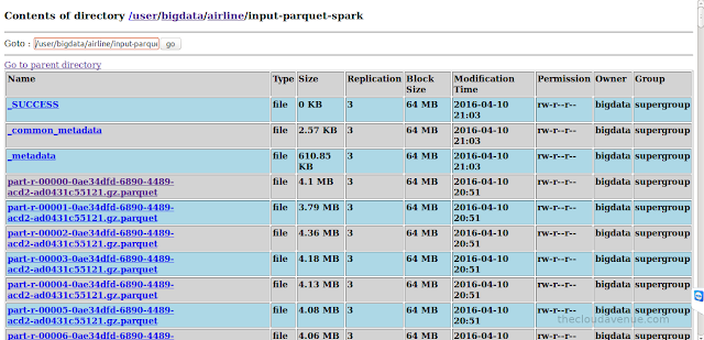
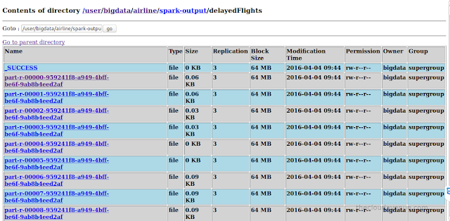
As seen in the below HDFS console, the number of Parquet files created by Spark were more than the number of files created by Hive and also smaller is size. This is not really efficient as HDFS has not be created to store smaller files. Here is an article from Cloudera on the same. Spark converted each block into a separate file in Parquet, but Hive combined multiple blocks into a single Parquet file. These are pros and cons of the way Hive and Spark have created the Parquet files which would be discussed in an upcoming blog.

Below is the comparison of the time taken and the size for both Hive and Spark. Note that these are got by using the out of the box setting with Hive and Spark and can be further fine tuned. The difference is the size if the default compression codes set in Hive and Spark.

PageRank on the English wiki data using MapReduce

PageRank is an iterative processing to find the relevancy of a web page in the world-wide-web. PageRank is one of the signal used by the search engine to figure out what to show at the top and what at the bottom of the search results. The `Data-Intensive Text Processing with MapReduce` has a very good description of what PageRank is and how to solve it in a MapReduce way.

As mentioned above PageRank is an iterative algorithm and MapReduce model is not good for iterative processing as the input and output of MapReduce in disk (from HDFS) which is really slow when compared to reading the data from the memory as in the case of Spark.

Anyway, working MapReduce code was available for the PageRank algorithm to process the Wiki data and so I thought of giving it shot. Here is the code and the description for the same. While iterating, if the difference between two iterations is small then the iterations are terminated. This logic is not implemented in the code.

Here is the data (english wiki) for the same. For those who don't have enough resources then a small wiki dump is also available for other languages.

It took 7 minutes short of 3 hours to process 52.58 GB of enhlish wiki data. The processing included a total of 7 MR programs. The first one for parsing the wiki xml data, 5 iterations using MR to calculate the PageRank and the final MR program for ordering the wiki pages based on the ranking.

Here is the configuration of the machine on which the wiki data has been processed.

 

Here is the folder structure in HDFS.

Here is the size of the input data.

Here is the size of the data after the first MR program (parsing the wiki). Not that the size of the data got decreased significantly, as we only need the list of web pages, the web pages it has connected to and the initial page ranking to start the PageRank algorithm.

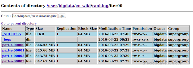
Here is the size of the final result, which is significantly small as only the webpage and the corresponding PageRank.

The file is a bit huge to open in gedit. So, head/tail is another way to look at the end of the file. Here is the screen for the same. Proud to see India in the top 10 list.

 

Here is the screenshot of the MapReduce console with the 7 MapReduce programs.

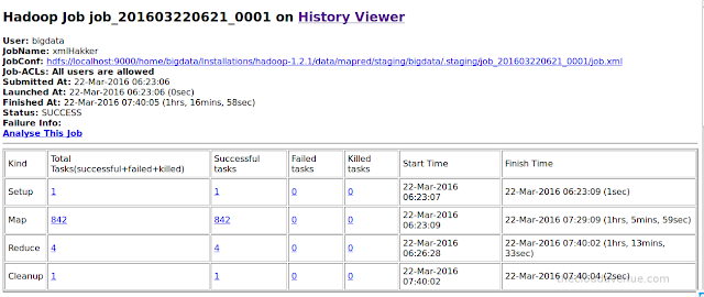
Here are the details of the first MapReduce program (xml parsing).

 Here are the details of the MapReduce program implementing a single MapReduce iteration for calculating the PageRank.

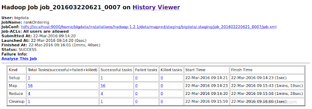
Here are the details of the MapReduce program implementing the sorting based on the PageRank.

The rational behind publishing so many screen shots is for the readers to get the different metrics for the processing of the English wiki data. Your mileage might very depending on the configuration of the machine and the size of the input wiki data used for the processing.

In the coming blogs, we will look into how to do the same think with Spark.

Analyzing the airline dataset with Spark/Python

The airline dataset in the previous blogs has been analyzed in MR and Hive, In this blog we will see how to do the analytics with Spark using Python. Programs in Spark can be implemented in Scala (Spark is built using Scala), Java, Python and the recently added R languages.

It took 5 min 30 sec for the processing, almost same as the earlier MR program. Not sure why Spark is not faster than MR as claimed, need to look into it a bit more. Here is the output (1, 2) of the Python program.

The Spark program is a bit more concise (short) when compared to the corresponding MR program. For those who are new to Spark, here is the Spark Python API.

from pyspark import SparkConf
from pyspark import SparkContext

import csv

def extractData(record) :

    #split the input record by comma
    splits = record.split(',')

    #extract the actual/scheduled departure time and the origin
    actualDepTime = splits[4]
    scheduledDepTime = splits[5]
    origin = splits[16]

    #1 delayed
    #0 don't know or not delayed
    delayed = 0

    # Check if the actual/scheduled departure time is a digit
    if actualDepTime.isdigit() & scheduledDepTime.isdigit():

        #if the flight got delayed or not
        if int(actualDepTime) > int(scheduledDepTime) :
            delayed = 1

    #return the origin and delayed status as a tuple
    return origin, delayed

#create the SparkConf() instance on which the different configurations can be done
conf = SparkConf().setMaster("spark://bigdata-server:7077")

#establish a connection to Spark
sc = SparkContext(conf = conf, appName = "flightDataAnalysis")

#load the input data
lines = sc.textFile("hdfs://localhost:9000/user/bigdata/airline/input")

#figure out the delayed flights and cache the data as it is being processed twice later
delayedFlights = lines.map(extractData).cache()

#get the delayed flights
delayedFlights.reduceByKey(lambda a, b : a + b).saveAsTextFile("hdfs://localhost:9000/user/bigdata/airline/spark-output/delayedFlights")

#get the total flights
totalFlights = delayedFlights.countByKey()

#totalFlights is dictionary. Iterate the same and write to a file
w = csv.writer(open("/home/bigdata/WorkSpace/PyCharm/AirlineDataset/output/totalFlights/totalFlights.csv", "w"))
for key, val in totalFlights.items():
    w.writerow([key, val])

As I mentioned in the previous blog, I do have a bit of high end machine for the data processing and below is resource usage in the Ubuntu system monitor when the above program is running. The CPU has 8 cores and all of them are running on full steam.

Now that we have seen how to convert CSV into Parquet format in the previous blog using Hive. We will look into how to process the same Parquet data with Spark using the DataFrame feature. After processing the data, the output is stored in the JSON format, so as to make it human readable.

from pyspark import SparkConf
from pyspark import SparkContext
from pyspark.sql import SQLContext

conf = SparkConf().setMaster("spark://bigdata-server:7077")
sc = SparkContext(conf = conf, appName = "flightDataAnalysis")
sqlContext = SQLContext(sc)

# load the parquet data
df = sqlContext.read.load("hdfs://localhost:9000/user/bigdata/airline/input-parquet")

# find the number of delayed flights per origin
delayedCount = df.filter(df.deptime > df.crsdeptime).groupBy(df.origin).count()

# Stored the delayed count as JSON
delayedCount.write.json("hdfs://localhost:9000/user/bigdata/airline/spark-output/delayedFlights")

Pycharm has been used to develop the program in Python and then executed in the Spark Standalone mode using the spark-submit command. As shown below it took 24 s to get the delayed flights.

 

Here is the output back in HDFS.

Here is the matrix, which shows the execution times with different softwares and formats on the same dataset and for the same problem.

In the future blogs, we will look into how to do the same processing with other softwares and also how to optimize it.

Twitter analysis with Pig and elephant-bird

Twitter analysis has been one of the popular blog on this site. Flume has been used to gather the data and then Hive has been used to do some basic analytics.  Performing the same with Pig had been pending for quite some time, so here it is.

The JSONLoader which comes with Pig can be used with Pig to load the JSON data from Flume. But, the problem with the JSONLoader is that that the entire scheme has to be specified as shown below. In the case of the Twitter data, the scheme becomes really huge and complex.

students = LOAD 'students.json'  USING JsonLoader('name:chararray, school:chararray, age:int');

So, I started using elephant-bird for processing the JSON date. With the JsonLoader from elephant-bird, there is no need to specify the schema. The JsonLoader simply returns a Pig map datatype and fields can be accessed using the JSON property name as shown below.

REGISTER '/home/bigdata/Installations/pig-0.15.0/lib/elephantbird/json-simple-1.1.1.jar'
REGISTER '/home/bigdata/Installations/pig-0.15.0/lib/elephantbird/elephant-bird-pig-4.3.jar'
REGISTER '/home/bigdata/Installations/pig-0.15.0/lib/elephantbird/elephant-bird-hadoop-compat-4.3.jar'

tweets = LOAD '/user/bigdata/tweetsJSON/' USING com.twitter.elephantbird.pig.load.JsonLoader('-nestedLoad') as (json:map[]);
user_details = FOREACH tweets GENERATE json#'user' As tweetUser;
user_followers = FOREACH user_details GENERATE (chararray)tweetUser#'screen_name' As screenName, (int)tweetUser#'followers_count' As followersCount;
user_followers_distinct = DISTINCT user_followers;
user_followers_sorted = order user_followers_distinct by followersCount desc;

DUMP user_followers_sorted;

The above program got converted into a DAG of 3 MapReduce programs and took 1 min 6 sec to complete, which is not really that efficient. It should be possible to implement the same using two MapReduce programs. I am not sure if there is any way to optimize the above Pig script. Any feedback, please let me know in the comments and I will try it out and update the blog.

The same data was proceed using Hive with the JSONSerDe provided by Cloudera as mentioned in the original blog. only a single MapReduce program was generated and it took 21 seconds to process the data, a drastic improvement over Pig using the elephant-bird library.

In the coming blogs. we will look a few other ways of processing the JSON data which is a very common format.

Analyzing the airline dataset with MR/Java

In the previous blog I introduced the Airline data set. I plan to get the results (total and delayed flights from different airports) using different Big Data softwares like Hadoop(MR), Hive, Pig, Spark, Impala etc and also with different formats of the data like Avro and Parquet. This will help the followers of the blog appreciate the different distributing computing software and models.

As usual there can be more than one of performing a particular task and a more efficient way. I have written the programs in a short span of time and will try to optimize them over time. Also, I will include as many comments as possible in the code, so as to make the code self explanatory.

Recently I have assembled a high configuration computer, which I like to call as a server :) with the below configurations. Ubuntu 14.04 64 bit has been installed on it. All the processing would be done on this server. It was fun looking for the right parts and assembling the computer. Initially I planned to buy an SSD instead of a Hard Disk, but the SSD were too expensive beyond the budget I planned.

Processor - AMD FX-6300 (FD6300WMHKBOX)
Mother Board - GIGABYTE GA-990XA-UD3
RAM - G.skill 2 * GB F3-12800CL10D-16GBXL
Hard Disk - Seagate 3.5 Inches Desktop 2 TB Hard Drive (ST2000DX001)

So, here is the MR program for calculating the total flight departures and the number of flight delays for the 20 years for each of the airport. Initially I wrote two MR programs, one for calculating the total flights and another for calculating the total delayed flights. This approach is not really efficient as the input data is parsed twice. So, I revamped the the program into one MR program.

Here is the MR Driver Code.

package AirlineDelaySinglePass;

import java.io.IOException;

import org.apache.hadoop.fs.Path;
import org.apache.hadoop.io.IntWritable;
import org.apache.hadoop.io.Text;
import org.apache.hadoop.mapred.FileInputFormat;
import org.apache.hadoop.mapred.FileOutputFormat;
import org.apache.hadoop.mapred.JobClient;
import org.apache.hadoop.mapred.JobConf;

public class AirlineDelayByStartTime {

 public static void main(String[] args) throws IOException {

  // Check if the number of parameters passed to program is 2
  if (args.length != 2) {
   System.err
     .println("Usage: AirlineDelayByStartTime <input path> <output path>");
   System.exit(-1);
  }

  // Create the JobConf instance and specify the job name
  JobConf conf = new JobConf(AirlineDelayByStartTime.class);
  conf.setJobName("Airline Delay");

  // First and second arguments are input and output folder
  FileInputFormat.addInputPath(conf, new Path(args[0]));
  FileOutputFormat.setOutputPath(conf, new Path(args[1]));

  // Specify the mapper and the reducer class
  conf.setMapperClass(AirlineDelayByStartTimeMapper.class);
  conf.setReducerClass(AirlineDelayByStartTimeReducer.class);

  // Specify the output key and value of the entire job
  conf.setOutputKeyClass(Text.class);
  conf.setOutputValueClass(IntWritable.class);

  // Specify the number of reducers tasks to run at any instant on a
  // machine, defaults to one
  conf.setNumReduceTasks(4);

  // Trigger the mapreduce program
  JobClient.runJob(conf);
 }
}

Here is the Mapper Code.

package AirlineDelaySinglePass;

import java.io.IOException;

import org.apache.commons.lang.StringUtils;
import org.apache.hadoop.io.IntWritable;
import org.apache.hadoop.io.LongWritable;
import org.apache.hadoop.io.Text;
import org.apache.hadoop.mapred.MapReduceBase;
import org.apache.hadoop.mapred.Mapper;
import org.apache.hadoop.mapred.OutputCollector;
import org.apache.hadoop.mapred.Reporter;

public class AirlineDelayByStartTimeMapper extends MapReduceBase implements
  Mapper<LongWritable, Text, Text, IntWritable> {

 public void map(LongWritable key, Text value,
   OutputCollector<Text, IntWritable> output, Reporter reporter)
   throws IOException {

  // Split the input line based on comma
  String[] pieces = value.toString().split(",");

  // Delayed 0 for ontime or NA, 1 for delayed
  int delayed = 0;

  // Get the origin which is the 17 field in the input line
  String origin = pieces[16];

  if (StringUtils.isNumeric(pieces[4])
    && StringUtils.isNumeric(pieces[5])) {

   // 5 DepTime actual departure time (local, hhmm)
   // 6 CRSDepTime scheduled departure time (local, hhmm)
   int actualDepTime = Integer.parseInt(pieces[4]);
   int scheduledDepTime = Integer.parseInt(pieces[5]);

   // if the flight has been delated
   if (actualDepTime > scheduledDepTime) {
    delayed = 1;
   }

  }

  // Send the Origin and the delayed status to the reducer for aggregation
  // ex., (ORD, 1)
  output.collect(new Text(origin), new IntWritable(delayed));

 }
}

Here is the Reducer Code

package AirlineDelaySinglePass;

import java.io.IOException;
import java.util.Iterator;

import org.apache.hadoop.io.IntWritable;
import org.apache.hadoop.io.Text;
import org.apache.hadoop.mapred.MapReduceBase;
import org.apache.hadoop.mapred.OutputCollector;
import org.apache.hadoop.mapred.Reducer;
import org.apache.hadoop.mapred.Reporter;

public class AirlineDelayByStartTimeReducer extends MapReduceBase implements
  Reducer<Text, IntWritable, Text, IntWritable> {

 private IntWritable value = new IntWritable();

 public void reduce(Text key, Iterator<IntWritable> values,
   OutputCollector<Text, IntWritable> output, Reporter reporter)
   throws IOException {

  // initialize the total flights and delayed flights
  int totalFlights = 0;
  int delayedFlights = 0;

  Text newKey = new Text();

  while (values.hasNext()) {

   // Delayed 0 for ontime or NA, 1 for delayed
   int delayed = values.next().get();

   // Increment the totalFlights by 1
   totalFlights = totalFlights + 1;

   // Calculate the number of delayed flights
   delayedFlights = delayedFlights + delayed;

  }

  // Create the key ex., ORD\t123
  newKey.set(key.toString() + "\t" + delayedFlights);

  // Create the value ex., 150
  value.set(totalFlights);

  // Pass the key and the value to Hadoop to write it to the final output
  output.collect(newKey, value);
 }
}

Here is the output of the MR program. This data can be joined with the Airport details (lat, long, name etc) to make it more readable and interesting. I could have written another MR program to do the join, but the size of the data set is so small that it doesn't make sense to use another MR program. We can simply use a spread sheet program or a database for joining of the data sets depending on the level of comfort.

Here is the time taken to run on my single node server. Note that the size of the airline data set is close to 12 GB and the processing is simple.

In the next blog I will post the code for doing the same with Spark.

Flight departure delays

The airline dataset is one of the interesting dataset which I came across recently. For 20 (1987 to 2008) years it has the actual/scheduled arrival/departure code, carrier code, flight number and a lot of other details.

From this information we can glean some interesting information like what is the best airline to travel, best time to travel. We can also mash with the weather data set to find out what sort of weather conditions cause flights to get delayed.

In this post I will publish what are the best and worst airport based on the number of delayed flights by departure. Chicago O'Hare International has the maximum number of departure delays (31,21,184). May be the total flights from O'Hare is huge, so I calculated the percentage (49.52%) of the number of departure delays (31,21,184) with the total number of flights (63,02,546) taking of from O'Hare. There are lot of factors influencing the flight delays, but delays are delays and O'Hare is one of the worst airport with respect to delays.



I have used MR programs for figuring out the same, which I would be publishing in the next blog after cleansing them up. For those interested to find out how the airport which is closet to them compares to other airports here is the data.